Forward Kinematics: Denavit-Hartenberg Convention
1 Introduction
In this post we look to develop the forward or configuration kinematic equations for a rigid robot of 6R (6 Revolute Joints) using the Denavit-Hartenberg convention. The forward kinematics problem is concerned with the relationship between the individual joints of a robot manipulator and the position and orientation of the tool or end-effector. Formally, the forward kinematics problem is to determine the position and orientation of the end-effector, given joint variable values of the robot. The joint variables are the angles between the links in the case of revolute or rotational joints, and the link extension displacement in the case of prismatic or sliding joints. The forward kinematics problem is to be contrasted with the inverse kinematics problem, which will be explored at another time, which is concerned with the determination of values for the joint variables that achieve a desired position and orientation for the end-effector of the robot.
2 Kinematics Fundamentals
To be able to fully define both the position and orientation of a robot end effector, one must determine linkage parameters such as link length, rotational link offset, and the two possible joint variables: link offset, and joint angle represented by symbols d, 𝛼, a, and 𝜃 respectively. The usage of either joint variable at each link depends on the joint type at each link. This paper deals with a 6R arm, and therefore the joint angle will be variable, and the link distance will be static (there exist no P joints). To perform forward kinematics, it is beneficial to establish orthogonal x,y,z coordinate frames at each of the various robot links to keep track of the different parameters as the system configuration changes.
3 Denavit-Hartenberg Convention
It is important to keep in mind that the choices of the various coordinate frames at each link are not unique. Thus it is possible for different engineers to derive differing frame assignments for the links on the robot by using different conventions.
While it is possible to carry out analysis using arbitrary frame assignments, the Denavit-Hartenberg convention makes frame selection systematic and consistent. By this convention, resultant calculations are also simplified as the DH convention follows two assumptions:
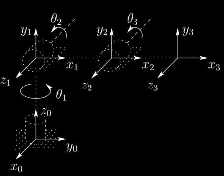
(DH1) The axis $x_i$ is ⟂ to the axis $z_{i-1}$
(DH2) The axis $x_i$ is coincident with the axis $z_{i-1}$
By following these assumptions, the need to reconcile a y-axis frame along every step is removed, and the forward kinematics problem becomes much easier to solve. As a part of the DH convention, the z axis of all frames are collinear with the joint axis, being the rotational axis in the case of a (R) revolute joint, and the linear actuation axis in the case of a (P) prismatic joint.
A robot manipulator with n joints will have n+1 links (Fig 3.1) since each joint connects two links. Joints are numbered 1 to n, and links are numbered 0 to n, starting from the base. By this convention, joint i connects link i-1 to link i. When joint i is actuated, link i moves.
With these frames, it is possible to derive a transformation matrix T, that expresses the position and orientation of frame $o_nx_ny_nz_n$ with respect to a base frame $o_ix_iy_iz_i$. $T_{j}^i$ is represented as a product of the separate transformation matrices that are based off of each link.
\[\begin{array}{c} T_{j}^{i}=A_{i+1} A_{i+2} \ldots A_{j-1} A_{j} \text { if } i<j \\ T_{j}^{i}=I \text { if } i=j \\ T_{j}^{i}=\left(T_{i}^{j}\right)^{-1} \text {if } j>i \end{array}\]By this definition, it is possible to derive the position and orientation of not just the end effector, but any of the frame origins established along one of the joints.
Each homogeneous transformation $A_i$ is of the form
\[\begin{aligned} A_{i} &=R_{n, \theta_{i}} \text { Trans }_{z, d_{i}} \text { Trans }_{x, a_{i}} R_{x, \alpha_{i}} \\ &=\left[\begin{array}{cccc} c_{\theta_{i}} & -s_{\theta_{i}} & 0 & 0 \\ s_{\theta_{i}} & c_{\theta_{i}} & 0 & 0 \\ 0 & 0 & 1 & 0 \\ 0 & 0 & 0 & 1 \end{array}\right]\left[\begin{array}{cccc} 1 & 0 & 0 & 0 \\ 0 & 1 & 0 & 0 \\ 0 & 0 & 1 & d_{i} \\ 0 & 0 & 0 & 1 \end{array}\right]\left[\begin{array}{cccc} 1 & 0 & 0 & a_{i} \\ 0 & 1 & 0 & 0 \\ 0 & 0 & 1 & 0 \\ 0 & 0 & 0 & 1 \end{array}\right]\left[\begin{array}{cccc} 1 & 0 & 0 & 0 \\ 0 & c_{\alpha_{i}} & -s_{\alpha_{i}} & 0 \\ 0 & s_{\alpha_{i}} & c_{\alpha_{i}} & 0 \\ 0 & 0 & 0 & 1 \end{array}\right] \\ &=\left[\begin{array}{cccc} c_{\theta_{i}} & -s_{\theta_{i}} c_{a_{i}} & s_{\theta_{i}} s_{\alpha_{i}} & a_{i} c_{\theta_{i}} \\ s_{\theta_{i}} & c_{\theta_{i}} c_{\alpha_{i}} & -c_{\theta_{i}} s_{\alpha_{i}} & a_{i} s_{\theta_{i}} \\ 0 & s_{\alpha_{i}} & c_{\alpha_{i}} & d_{i} \\ 0 & 0 & 0 & 1 \end{array}\right] \end{aligned}\]Thus the position and orientation of the end effector with respect to the base frame is given by homogeneous transformation matrix
\[\begin{aligned}\begin{array}{c} H=T_{n}^0=A_{1} \cdots A_{n} \end{array}\end{aligned}\]4 Summary
We may summarize the above procedure based on the D-H convention in the following algorithm for deriving the forward kinematics for any manipulator
Step 4.1: Locate and label the joint axes $z_0$, … ,$z_{n−1}$.
Step 4.2: Establish the base frame. Set the origin anywhere on the $z_0$-axis. The $x_0$ and $y_0$ axes are chosen conveniently to form a right-hand frame. For $i = 1, … , n − 1$, perform Steps 3 to 5.
Step 4.3: Locate the origin $O_i$ where the common normal to $z_i$ and $z_{i−1}$ intersects $z_i$. If $z_i$ intersects $z_{i−1}$ locate $O_i$ at this intersection. If $z_i$ and $z_{i−1}$ are parallel, locate $O_i$ in any convenient position along $z_i$.
Step 4.4: Establish $x_i$ along the common normal between $z_{i−1}$ and $z_i$ through $O_i$, or in the direction normal to the $z_{i−1} − z_i$ plane if $z_{i−1}$ and $z_i$ intersect.
Step 4.5: Establish $y_i$ to complete a right-hand frame.
Step 4.6: Establish the end-effector frame $o_nx_ny_nz_n$. Assuming the n-th joint is revolute, set $z_n = a$ along the direction $z_{n−1}$. Establish the origin $O_n$ conveniently along $z_n$, preferably at the center of the gripper or at the tip of any tool that the manipulator may be carrying. Set $y_n = s$ in the direction of the gripper closure and set $x_n = n$ as $s × a$. If the tool is not a simple gripper set $x_n$ and $y_n$ conveniently to form a right-hand frame.
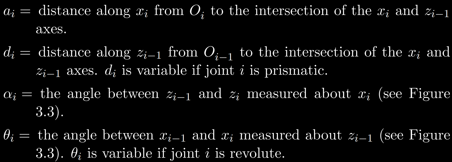
Step 4.7: Create a table of link parameters $a_i, d_i, α_i, θ_i$
Step 4.8: Form the homogeneous transformation matrices Ai by substituting the above parameters into (3.4).
Step 4.9: Form$ \begin{array}{c} H=T_{n}^0=A_{1} \cdots A_{n} \end{array}$. This then gives the position and orientation of the tool frame expressed in base coordinates.
5 Specific Embodiment of DH Convention on a 6R Example
By going through the steps outlined in section 4, one may arrive at the resultant $H_{n}^0$ matrix for a rigid robot with any number of joints and any combination of joint types. In this section we attempt the outlined steps 4.1 through 4.9 on a specific example of a designed 6R robotic arm.
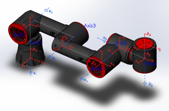
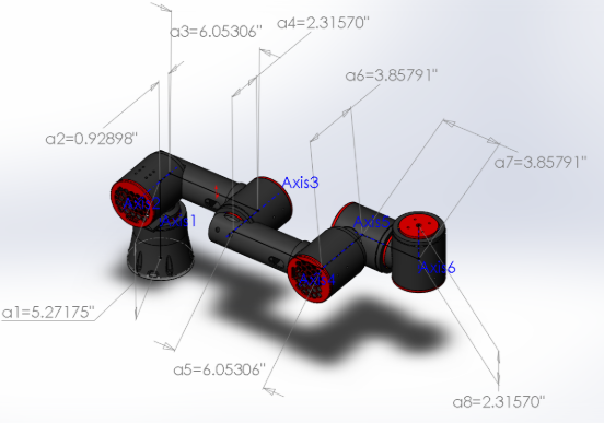
In (Fig 5.1), it is evident that steps 4.1 and 4.2 are completed, and that 4.3-4.5 are satisfied for each link. Step 4.1 is simply the convention that the z axis at any link i should be collinear with the joint axis. Step 4.2 is the establishment of the base frame, which is grounded in our case and defined as the origin at $x_0y_0z_0$. Steps 4.3-4.5 are simply the assumptions of the Denavit-Hartenberg convention stated by DH1 and DH2 in section 3. Step 4.6 is also satisfied and is illustrated in (Fig 5.1) and the end effector frame origin is assigned as the point coplanar to and centered on the actuator surface. There exists no explicit joint at frame $x_6y_6z_6$, however, it is actuated by Axis6. $a_i, d_i, α_i, θ_i$
| $i$(Frame) | $θ_i$ | $α_i$ | $a_i$ | $d_i$ |
|---|---|---|---|---|
| 1 | $θ_1$ | $90$ | $0$ | $a_1$ |
| 2 | $θ_2$ | $0$ | $a_3$ | $a_4-a_2$ |
| 3 | $θ_3$ | $0$ | $a_5$ | $0$ |
| 4 | $θ_4$ | $90$ | $0$ | $-a_6$ |
| 5 | $θ_5$ | $90$ | $0$ | $a_7$ |
| 6 | $θ_6$ | $0$ | $0$ | $a_8$ |
By completing Table 5.3 we have completed step 4.7. Notice that frame 0 of $x_0y_0z_0$ is not present, as all of the parameters within the table are based on the relation between frame $i$, and frame $i-1$. Thus, with frame 0 having no preceding frame to reference, it is not present within the table, but instead we look to establish parameters of frame 1 in relation to frame 0 in the first data row of the table.
Since the robot is of 6R, we must include variable parameters that account for the freely rotating joints. These variables are present in the $θ_i$ column, since per the D-H convention, $θ_i$ is a variable if joint $i$ is revolute. To verify that the table was done correctly, all joint variables ( $θ_1$ … $θ_6$ ) as well as all link lengths ($d_i$) and link offsets ($a_i$) (a1-a8) should be accounted for in the table.
Next, we must establish each transformation matrix $A_i$, which describes the transformational relation between frame $i$, and frame $i-1$, for each frame. This becomes difficult to compute by hand so we may use computational tools such as python to aid us.
\[\begin{aligned}\left[\begin{array}{cccc} c_{\theta_{i}} & -s_{\theta_{i}} c_{a_{i}} & s_{\theta_{i}} s_{\alpha_{i}} & a_{i} c_{\theta_{i}} \\ s_{\theta_{i}} & c_{\theta_{i}} c_{\alpha_{i}} & -c_{\theta_{i}} s_{\alpha_{i}} & a_{i} s_{\theta_{i}} \\ 0 & s_{\alpha_{i}} & c_{\alpha_{i}} & d_{i} \\ 0 & 0 & 0 & 1 \end{array}\right] \end{aligned}\]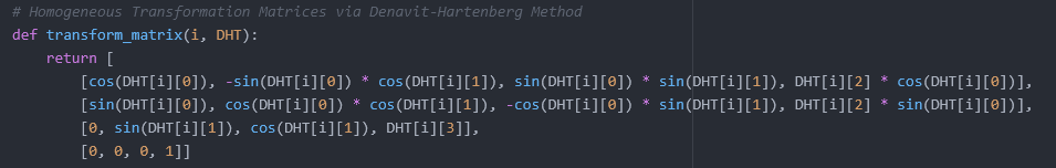
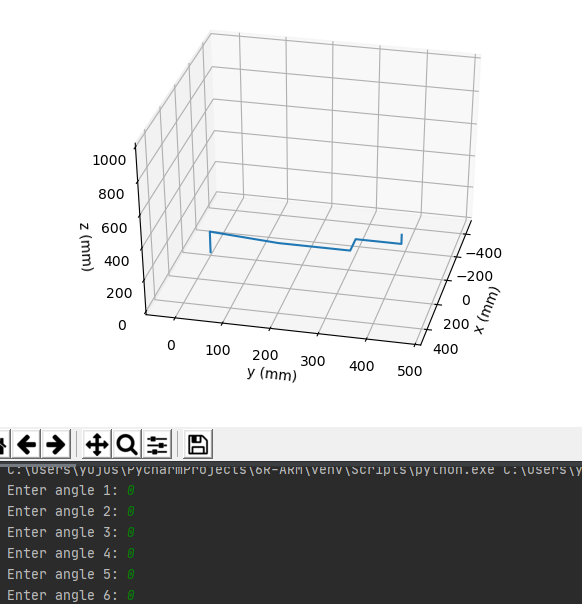
Using the determined matrices for each frame, we may then dot them all together in the order of $A_{1} \cdots A_{6}$ to determine transform matrix $H_6^0$, which describes the end effector position and orientation in relation to the base frame.
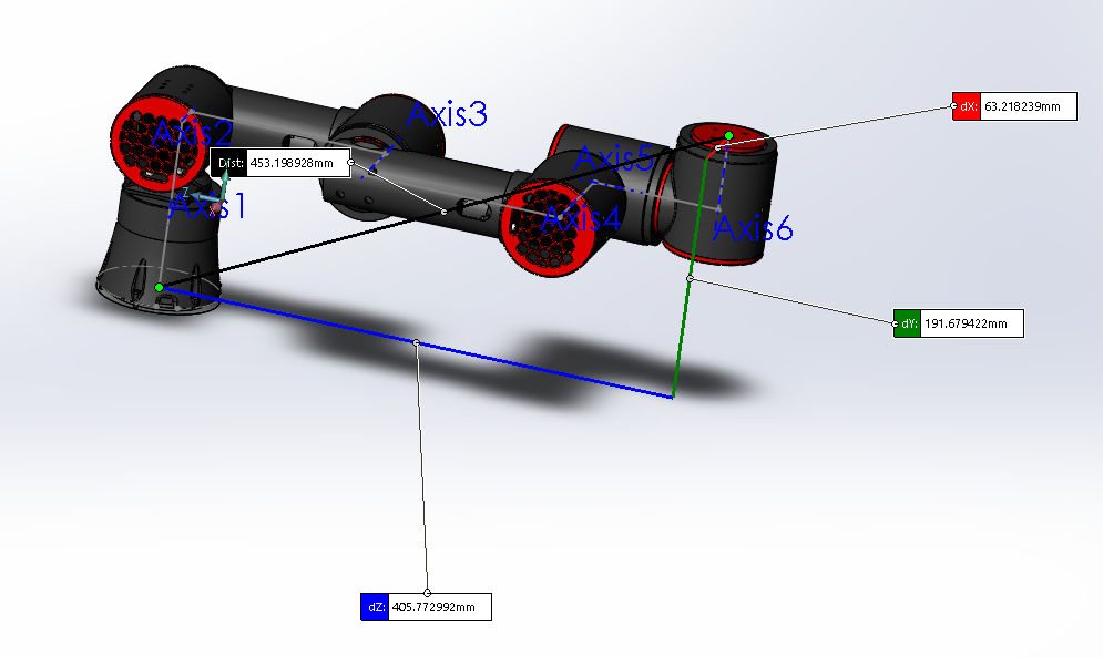
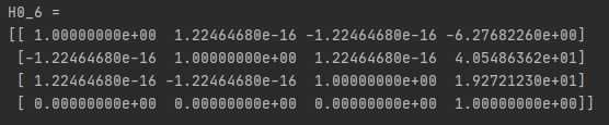
The numbers match closely! (Variance is due to hand-placed and orientated arm links in CAD model). The -6.3cm value in the python console is correctly negative. Base frame (grounded frame) utilizes an $x_0$ axis frame pointing in the opposite direction (Fig 5.6). As detailed in (Fig 5.7), end effector position is detailed by the first 3 entries of the final column of the matrix. End effector orientation is reconciled by the first 3x3 rows and columns of the matrix.