


1University of California, Berkeley 2Stanford University 3XDOF
*Equal contribution. †Corresponding author: yujustin@berkeley.edu



Which Data is Worth Imitating?
On long-horizon tasks, collecting high-quality data becomes increasingly difficult. Even skilled humans make mistakes on challenging tasks, leaving low-quality segments scattered throughout otherwise-successful demonstrations. This pushes roboticists toward data curation: deciding which data is actually worth imitating.
Frame-level curation methods estimate progress inside a demonstration and filter or re-weight individual action chunks by how much they advance the task. SARM and ARM learn this from human-annotated labels on long-horizon T-shirt folding.
A common self-supervised signal in progress reward modeling is the fraction of the trajectory completed so far, the normalized frame index1. Normalized elapsed time can be a useful proxy for task progress when progress is approximately linear within each demonstration, even if some demonstrations are faster than others. But pauses, retries, and uneven pacing break this correspondence: halfway through one demonstration may represent a very different task stage than halfway through another.
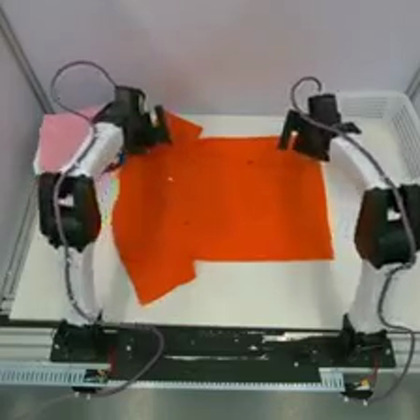
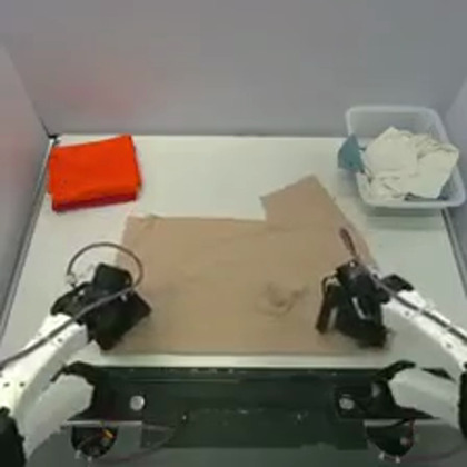
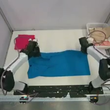
All three frames sit at 50% of their video, yet show different stages of the task. We conjecture that supervising on normalized elapsed time injects noise into task progress estimation models, an issue exacerbated for longer horizon tasks.
WARP-RM produces a dense, signed, per-frame progress velocity signal straight from the demonstrations, with no human annotations required.
The progress signal
The curve under each video is WARP-RM's output: a dense, per-frame signed progress velocity, \(\hat{v}_{t}\). A value near one represents the reference pace defined by the training labels; values near zero suggest stagnation, and negative values suggest regression. Click anywhere on the curve to scrub the video.
Episodes A and B play real teleoperated episodes while the curve shows the dense per-frame predicted signed progress magnitude \(\hat{v}_{t}\): positive for forward task progress and negative for regression. Click on the curve to scrub through the video.
Method
Each training example is a window of 32 frames sampled from a successful demonstration. Per-step playback speeds are drawn from an AR(1) process in log-space, so the clip drifts smoothly between slow-motion and fast-forward, and the total span the window covers is itself sampled, anywhere from a short stretch seen in slow motion to most of the demonstration skimmed quickly. Some steps run in reverse (Poisson-sampled), and the whole window is flipped with probability 0.5. Each sampled frame's signed temporal offset from the window's first frame, normalized by the reference stride and window length, supplies a self-supervised relative-progress target.
A frozen DINOv3 ViT-B/16 + 12-layer bidirectional transformer head outputs a per-frame categorical distribution over cumulative progress. Its temporal derivative gives the velocity \(\hat{v}_{t}\):
\(\hat{v}\) ≈ 1 → reference pace, \(\hat{v}\) ≈ 0 → stagnating, \(\hat{v}\) < 0 → regressing
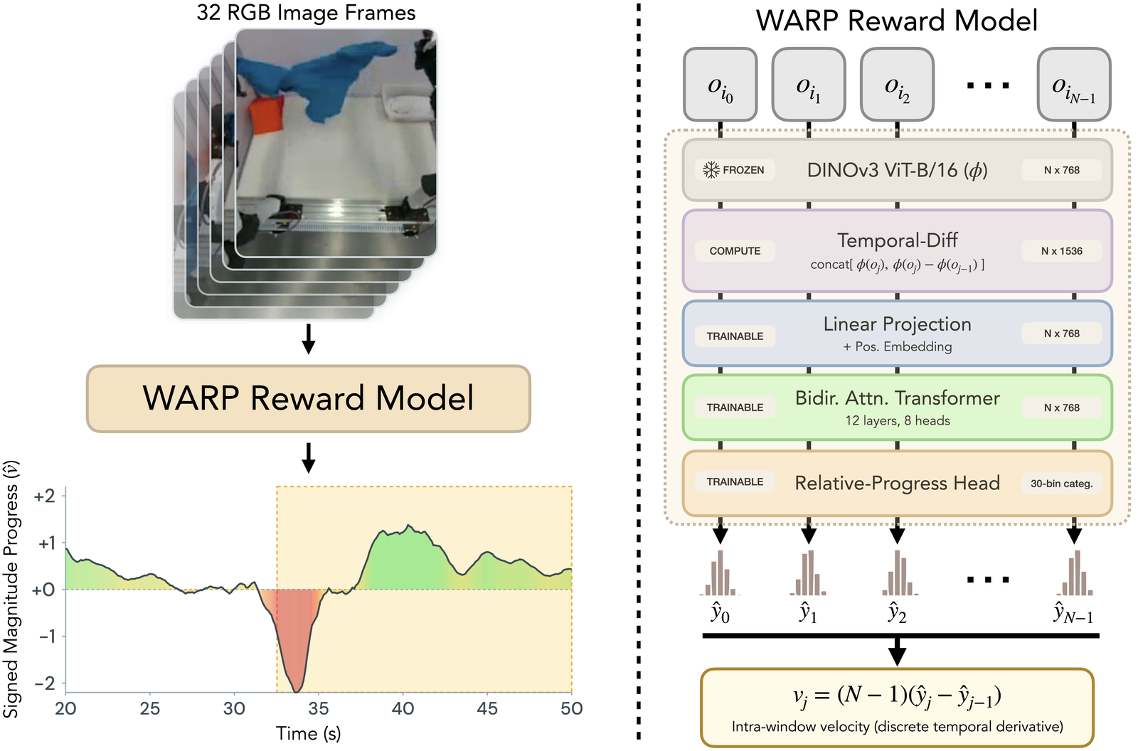
For each training chunk, gate on the predicted velocity at its terminal frame. With \(\tau = 1.0\), only chunks whose predicted terminal progress velocity exceeds the reference pace are kept, and each is weighted continuously by its velocity:
\( w \;=\; \hat{v}_{\mathrm{end}} \cdot \mathbf{1}\{\,\hat{v}_{\mathrm{end}} > \tau\,\} \)
Data
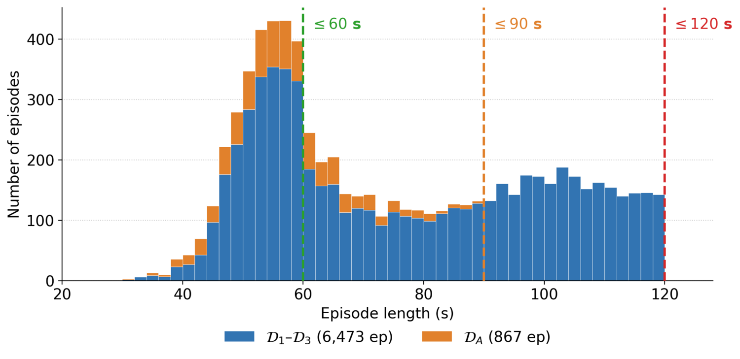
Our policy-training data is drawn from a dataset of around 140 hours of successful, unannotated human-teleoperated T-shirt-folding demonstrations. On this task, episode length is a coarse proxy for execution efficiency: longer episodes tend to contain more hesitations, retries, and recoveries. To evaluate robustness as progressively more inefficient behavior is admitted into training, we define three nested, length-filtered tiers: \(\mathcal{D}_{1}\) (≤ 60s): 2,427 episodes (36.1 hours), \(\mathcal{D}_{2}\) (≤ 90s): 4,124 episodes (71.3 hours), and \(\mathcal{D}_{3}\) (≤ 120s): 6,473 episodes (139.7 hours). Policies are trained on the same underlying demonstrations, either with uniform weighting (vanilla BC) or WARP-based progress reweighting. A single WARP-RM model is used across all tiers: it is trained once on a fixed reference subset \(\mathcal{D}_{\mathrm{RM}}\), the shortest demonstrations (≤ 59.8s, 1,950 episodes), providing a clean reference signal for the canonical execution pace (\(\hat{v} = 1\)). For baseline comparisons, SARM requires human annotations, so an annotated supplement \(\mathcal{D}_{A}\) (867 expert demonstrations, 13.9 hours) is added, forming the augmented datasets \(\mathcal{D}_{4} = \mathcal{D}_{1} \cup \mathcal{D}_{A}\) and \(\mathcal{D}_{5} = \mathcal{D}_{2} \cup \mathcal{D}_{A}\); WARP-RM and all other baselines treat \(\mathcal{D}_{A}\) as unannotated.
| Dataset / tier | Filter | Episodes | Total hours |
|---|---|---|---|
| \(\mathcal{D}_{1}\) | policy training, ≤ 60s | 2,427 | 36.1 |
| \(\mathcal{D}_{2}\) | policy training, ≤ 90s | 4,124 | 71.3 |
| \(\mathcal{D}_{3}\) | policy training, ≤ 120s | 6,473 | 139.7 |
| \(\mathcal{D}_{A}\) | annotated supplement (SARM) | 867 | 13.9 |
| \(\mathcal{D}_{\mathrm{RM}}\) | WARP-RM reference, ≤ 59.8s | 1,950 | 28.7 |
Real-World Policy Rollouts
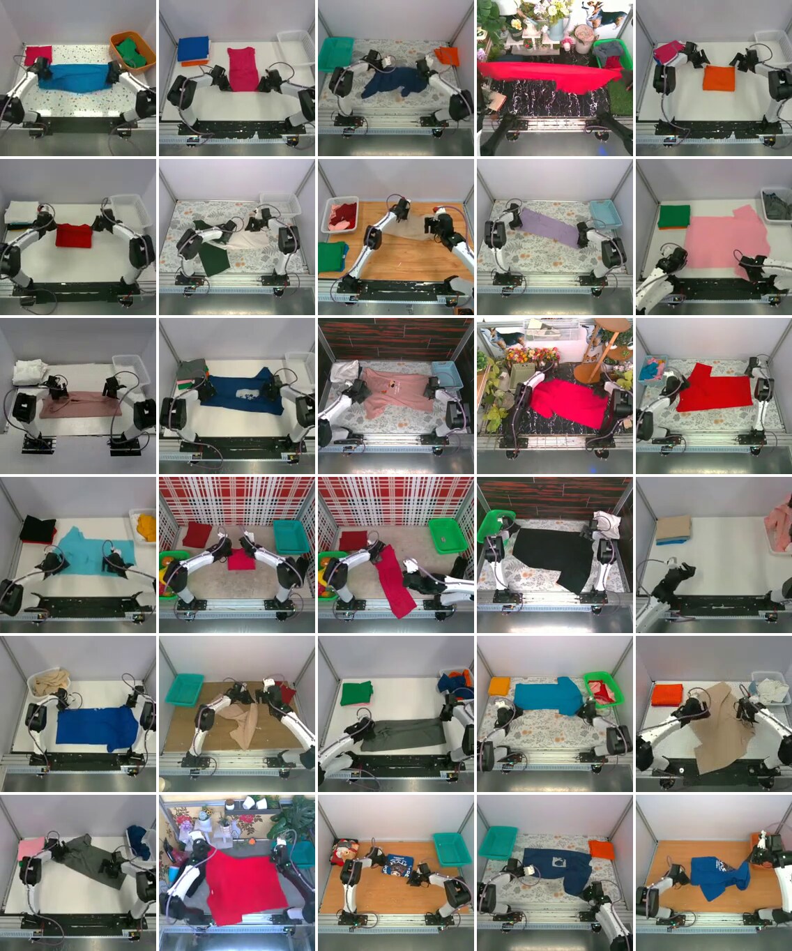
Across 380 real-world trials of T-shirt folding from a crumpled start, WARP-BC succeeds more often, and finishes faster when it does, than vanilla BC and the other baselines trained on the same dataset. Each grid below plays all 20 evaluation trials for one tier at once, in a 4×5 layout. Use the selector to switch between the three demonstration tiers.
Videos played at 1× speed.
Quantitative Results
Cross-tier results on T-shirt folding
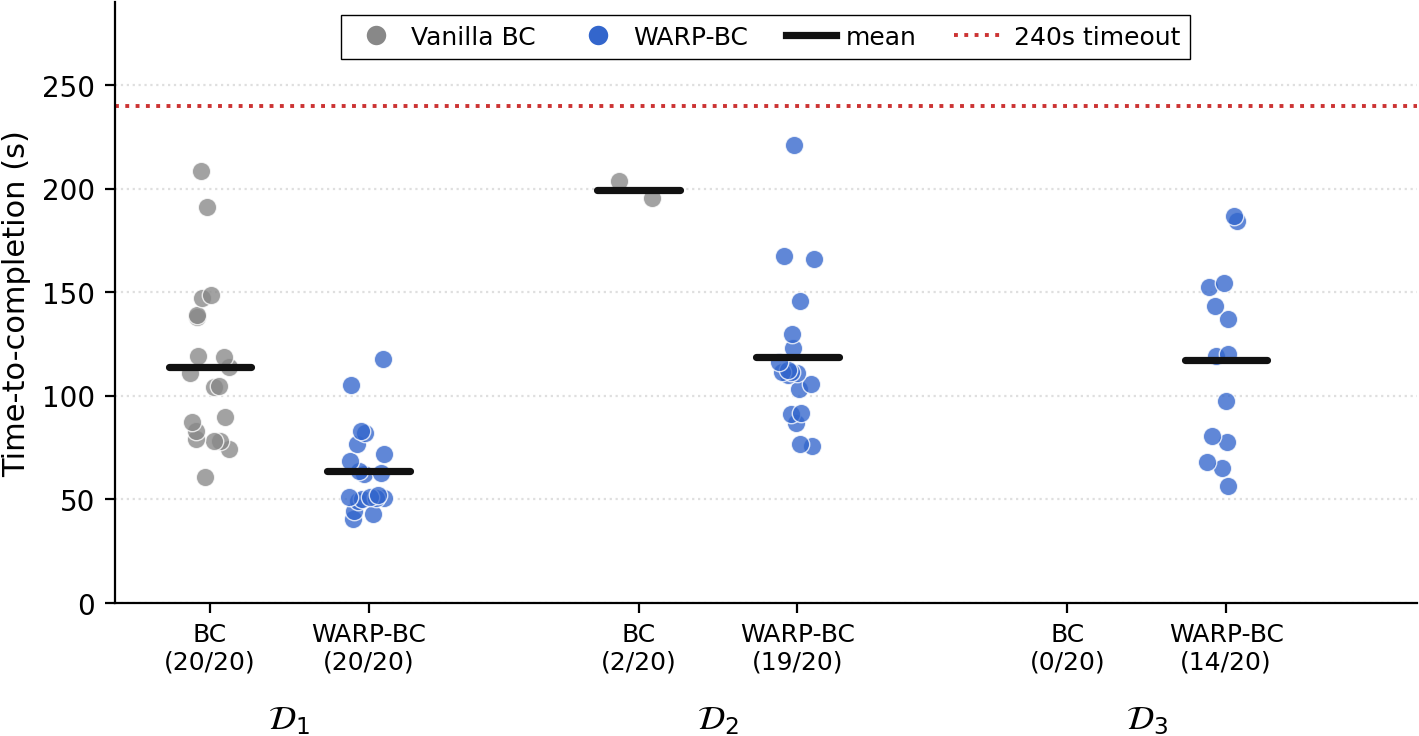
All policies are evaluated on 20 trials of T-shirt folding from a crumpled start with a 240s timeout. Mean time-to-completion (TTC) is reported over successful trials only. As the training pool admits more suboptimal demonstrations, vanilla BC degrades sharply while WARP-BC stays robust.
Full table
| Method | Metric | \(\mathcal{D}_{1}\) (≤60s) | \(\mathcal{D}_{2}\) (≤90s) | \(\mathcal{D}_{3}\) (≤120s) |
|---|---|---|---|---|
| Vanilla BC | Success ↑ | 20/20 | 2/20 | 0/20 |
| Mean TTC (s) ↓ | 113.8 | 199.0 | N/A | |
| Throughput (/hr) ↑ | 31.6 | 1.5 | 0.0 | |
| Action Chunks Kept | 100% | 100% | 100% | |
| WARP-BC | Success ↑ | 20/20 | 19/20 | 14/20 |
| Mean TTC (s) ↓ | 63.9 | 118.8 | 117.4 | |
| Throughput (/hr) ↑ | 56.3 | 27.4 | 16.3 | |
| Action Chunks Kept | 35.7% | 34.4% | 22.5% |
Matched baseline comparisons
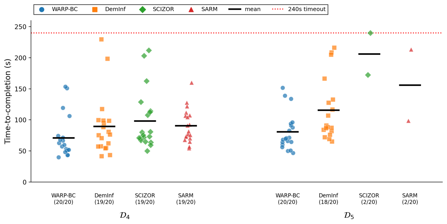
Because SARM requires human-annotated subtask boundaries, all methods are evaluated on the augmented corpora \(\mathcal{D}_{4} = \mathcal{D}_{1} \cup \mathcal{D}_{A}\) and \(\mathcal{D}_{5} = \mathcal{D}_{2} \cup \mathcal{D}_{A}\), where \(\mathcal{D}_{A}\) is the annotated supplement (treated as unannotated by every method except SARM). WARP-BC sustains the highest throughput on both tiers and ties or leads on success, all without the human labels SARM needs. SARM and SCIZOR collapse on the noisier \(\mathcal{D}_{5}\), while DemInf stays robust on success but at lower throughput.
Full table
| Method | Metric | \(\mathcal{D}_{4}\) | \(\mathcal{D}_{5}\) |
|---|---|---|---|
| SARM | Success ↑ | 19/20 | 2/20 |
| Mean TTC (s) ↓ | 90.5 | 156.0 | |
| Throughput (/hr) ↑ | 34.9 | 1.55 | |
| Action Chunks Kept | 78.5% | 66.6% | |
| DemInf | Success ↑ | 19/20 | 18/20 |
| Mean TTC (s) ↓ | 89.6 | 115.8 | |
| Throughput (/hr) ↑ | 35.2 | 25.3 | |
| Action Chunks Kept | 45.6% | 33.7% | |
| SCIZOR | Success ↑ | 19/20 | 2/20 |
| Mean TTC (s) ↓ | 98.4 | 206.2 | |
| Throughput (/hr) ↑ | 32.4 | 1.5 | |
| Action Chunks Kept | 77.9% | 66.7% | |
| WARP-BC | Success ↑ | 20/20 | 20/20 |
| Mean TTC (s) ↓ | 71.2 | 80.7 | |
| Throughput (/hr) ↑ | 50.6 | 44.6 | |
| Action Chunks Kept | 45.6% | 33.7% |
Another Task: Bottle-in-Bin Placement
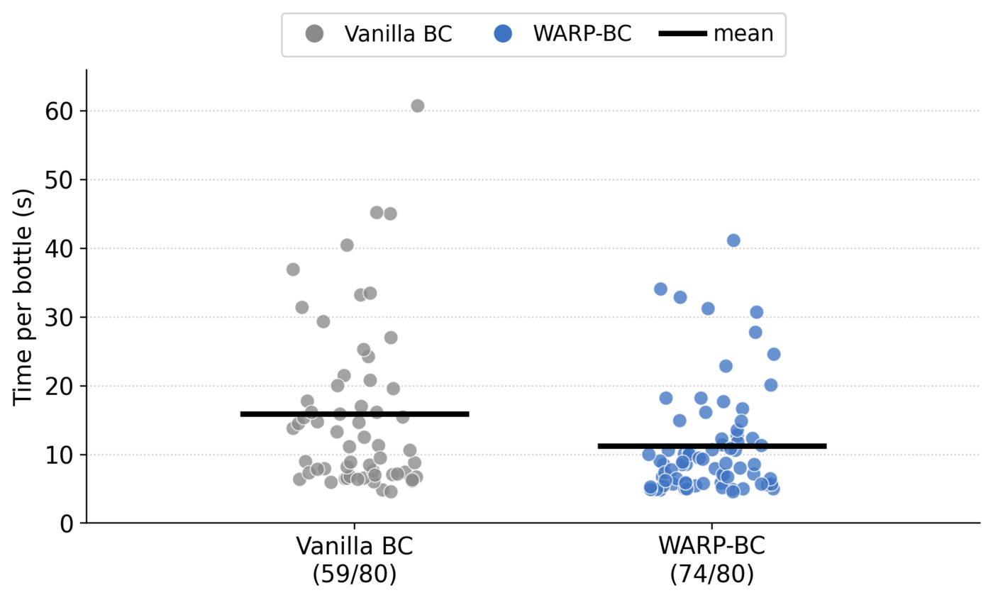
Beyond folding, we run the same recipe on a bottle-in-bin placement task with the same bimanual robot. Each trial drops four bottles into a bin under a 90 s timeout (20 trials, 80 bottles per policy), and both policies train on the same demonstrations.
Each grid plays all 20 trials at 1× speed, fully autonomous.
Full table
| Method | Bottles placed ↑ | Time / bottle (s) ↓ | Throughput (/hr) ↑ | Act. Chunks Kept |
|---|---|---|---|---|
| Vanilla BC | 59 / 80 | 15.9 | 147.8 | 100% |
| WARP-BC (Ours) | 74 / 80 | 11.3 | 237.8 | 30.6% |
WARP-BC places more bottles (74/80 vs 59/80), cuts mean per-bottle time from 15.9→11.3 s, and improves throughput 1.6×.
Simulation: 512 Paired Scenes
On simulated bottles-in-bin, WARP-BC clears all six bottles in 25.0% of scenes versus 9.4% for vanilla BC (2.7×) while retaining 31.5% of action chunks. It also increases throughput from 237 to 290 bottles/hour (22%) and places 4.533 bottles per scene versus 3.885.
Each method is evaluated on the same 512 scene seeds, with six bottles per scene and a nominal 60-second horizon. Curation methods share demonstrations, policy architecture, training-step budget, and a 31.5% retention budget; vanilla BC uses all the data.
Full table
| Method | Data kept | Bottles/scene ↑ | Throughput (/hr) ↑ | All 6 cleared ↑ |
|---|---|---|---|---|
| Vanilla BC | 100% | 3.885 | 237 | 9.4% |
| Random | 31.5% | 3.770 | 230 | 10.9% |
| ReWiND | 31.5% | 3.781 | 231 | 9.4% |
| SARM (oracle) | 31.5% | 4.191 | 265 | 20.5% |
| WARP-BC (IID) | 31.5% | 4.285 | 269 | 18.9% |
| SCIZOR | 31.5% | 4.299 | 270 | 19.1% |
| DemInf | 31.5% | 4.332 | 271 | 18.8% |
| WARP-BC | 31.5% | 4.533 | 290 | 25.0% |
SARM (oracle) uses stage boundaries from simulator state. The rollout executes 1,800 control steps (61.2 seconds at the configured timestep). Values are from the published simulation table; paired n=512 traces for vanilla BC and WARP-BC are public.
Reproduce the Simulation Experiments
The WARP simulation pipeline is reproducible end to end from public artifacts. Start from the released demonstrations, train your own reward model and policy, then run the simulator and scorer using the documented recipe and pinned companion repositories.
- Get the data. Download the LeRobot demonstrations, scene assets, and full-state supplement.
- Train and score with WARP-RM. Use the reward-model code to learn progress and inject per-frame rewards, or start with the released reward-model checkpoint.
- Curate and train the policy. Apply the WARP chunk gate and train π0 with the companion OpenPI code. Released policy checkpoints also support evaluation without retraining.
- Roll out and score. Run the MuJoCo-Warp evaluator on paired scenes and inspect the published n=512 rollout traces.
Fresh training and rollouts are stochastic; compare aggregate results. The separate n=128 trace self-test verifies the scorer against a fixed replay set. The guide documents baseline-specific reproduction limits and pretrained-model access terms.
Ablations
All ablations are run on dataset \(\mathcal{D}_{2}\). Kept-train-samples reports the fraction of action chunks that survive the weighting filter.
Full table
| Variant | Success ↑ | Mean TTC (s) ↓ | Throughput (/hr) ↑ | Action Chunks Kept |
|---|---|---|---|---|
| Weighting function | ||||
| \(\tau = 0\) | 3/20 | 201.4 | 2.3 | 97.0% |
| \(\tau = 1\), max = 1 (binary) | 16/20 | 139.6 | 18.0 | 34.4% |
| \(\tau = 1\), continuous — WARP | 19/20 | 118.8 | 27.4 | 34.4% |
| RA-BC aggregation strategy | ||||
| Mean over 1s action chunk | 15/20 | 127.0 | 17.4 | 34.0% |
| Mean over 1s, one-chunk offset | 14/20 | 124.2 | 15.9 | 34.3% |
| Terminal \(\hat{v}_{end}\) — WARP | 19/20 | 118.8 | 27.4 | 34.4% |
| WARP sampler | ||||
| IID log-normal | 18/20 | 131.0 | 22.8 | 28.7% |
| AR(1) process — WARP | 19/20 | 118.8 | 27.4 | 34.4% |
- Progress reward models that supervise on this signal include Robometer, ReWiND, and ProgressVLA. Each regresses a frame's normalized position in the trajectory, from the first frame to the last, as its per-frame progress target.
Citation
@article{yu2026warp,
  title={WARP-RM: A Warp-Augmented Relative Progress Reward Model for Data Curation},
  author={Yu, Justin and Goldberg, Andrew and Kondap, Kavish and El-Refai, Karim and Ransing, Ethan and Chen, Qianzhong and Schwager, Mac and Shentu, Fred and Wu, Philipp and Goldberg, Ken},
  journal={arXiv preprint arXiv:2606.28320},
  year={2026}
}